Financial Modeling

Frequency distribution

Frequency distributions display the frequency of outcomes for a specified sample and time period. The distribution plots the number of occurrences for a data set using a histogram.

Frequency distributions provide a concise, visual representation of a collection of data points and organize seemingly random information into a summarized presentation.

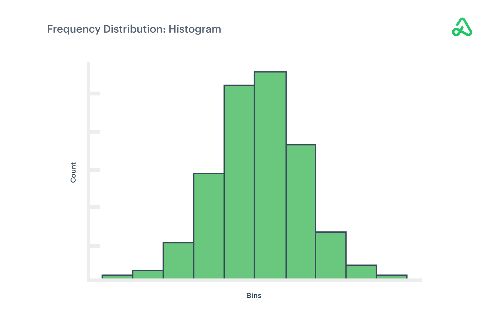
Frequency distribution demonstrates valuable information for an observed group, such as the median, mean, high and low extremes, standard deviations, outliers, and averages.

Frequency distributions are often the starting point for a more in-depth analysis of variance and standard deviation for a data set.

Variability

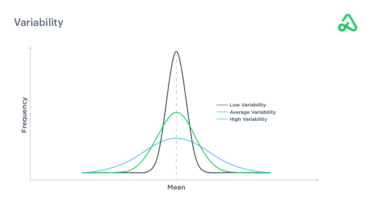
Variability measures how widely data differs from the average in a statistical study. 

Less variability translates to a smooth equity curve without large periods of volatility and drawdowns. More variability typically has more risk but can be offset by the potential for larger returns. Variability is frequently measured by variance, which is the amount a variable differs from its expected value.

Variance

Variance is a measure of dispersion for a set of data. Variance measures the deviation from an average value. The larger the variance, the further the data points are from the average of all the data.

To calculate the variance for a sample, find the average of the data set, then subtract the actual return for each data point from the average return to measure how far each data point deviates from the expected value. Square each of these deviations and then add the squared deviations. Finally, divide the sum of the squared deviations by the number of values in the data set, minus one.

Variance has two primary uses in finance.

First, variance is used to optimize portfolio allocation. A portfolio containing assets with high variance will likely be subject to large swings in volatility and risk. Variance can be used to analyze multiple assets’ performance to determine the best fit for a portfolio based on risk tolerance.

Second, investors use variance to determine the standard deviation of price movements and the implications those changes will have on a portfolio. The square root of the variance is the standard deviation, and standard deviation is a key variable in many financial models.

Variance is less intuitive than the standard deviation as it is measured in squared units.

Standard deviation

Standard deviation is a measure of the distribution of data points relative to their average value.

Standard deviation is applied to the average annual return of an investment to measure the investment’s volatility. Actual returns are compared to the average return to determine how much the actual returns deviate from expectations.

Standard deviation is not to be confused with mean absolute deviation, which is simply the sum of the differences between observations and the mean. The standard deviation takes those differences and squares them, ultimately summing then taking the square root. The squaring step in this math places a larger weight on large observations. 

Standard deviation is the square root of the variance and will show how much an asset tends to move up or down over a defined period. The higher the standard deviation, the larger the range of movement for an asset’s price over a period of time, and, thus, the wider the distribution of expected outcomes.

Stocks with a lower standard deviation are less volatile and will have lower implied risk.

Standard deviation relies on a normalized distribution and assumes all unpredictability as a risk. Standard deviation can show if returns are normally distributed or deviate from an expected rate of return.

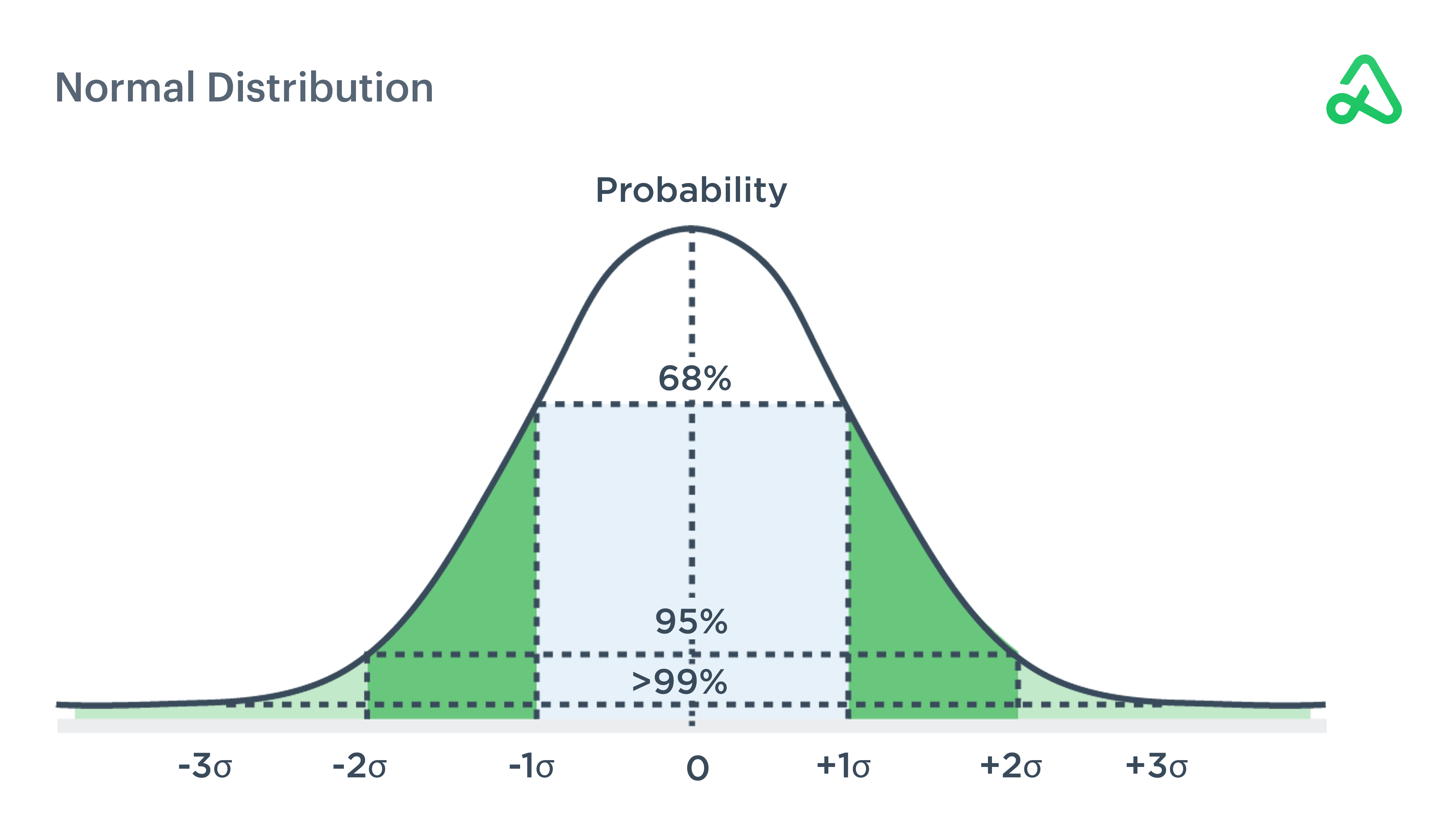
With a normal distribution, one standard deviation accounts for 68% of the data measured. Two standard deviations represent 95% of expected outcomes, and three standard deviations contain approximately 99% of expected outcomes for a normal distribution.

Skew

If the shape of the distribution differs from a normal distribution where the mean and median are not centered, it is said to be skewed. A normal distribution is symmetrical, while a skewed distribution is pulled to one side or the other and appears imbalanced.

In a normal distribution, the mean, median, and mode are all the same. If the mean is skewed to the right, or above, the median, it is said to have a positive skew and will appear to have a “tail” that extends farther to the right from the center of the graph.

If the mean is skewed to the left, or below, the median, it is said to have a negative skew and will appear to have a “tail” that extends farther to the left from the center of the graph.

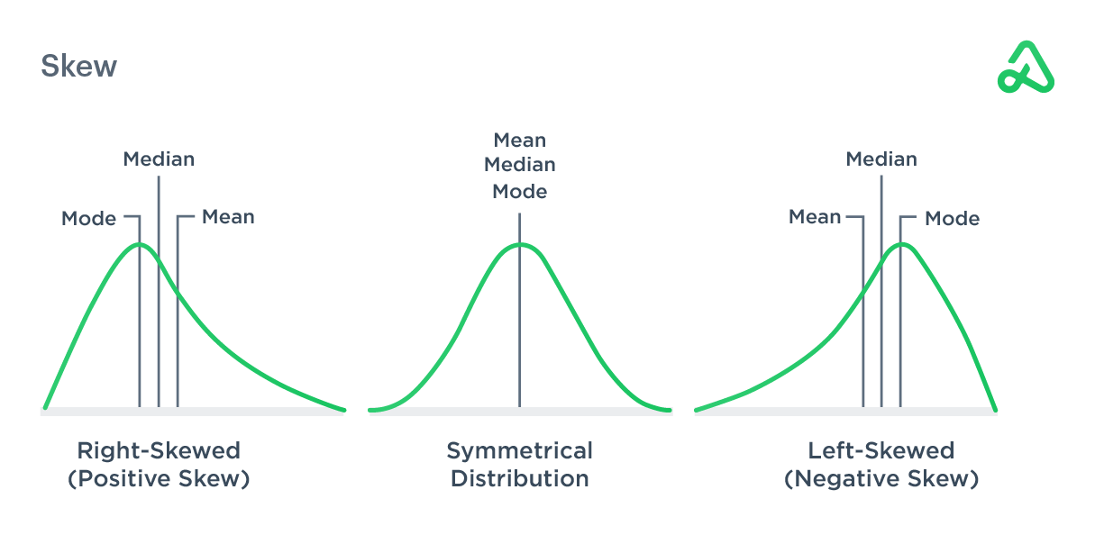
In finance, if the distribution has a positive skew, the investment has exceeded the expectations of a normal return for a specified period of time. Left-skewed or negatively skewed distributions have outliers at low-value levels while right-skewed or positively skewed distributions have outliers at high-value levels.

Distributions

Distributions demonstrate the probability of a specific outcome for a set of variables. Distributions are typically displayed as curves on a graph. The curve depicts the distribution of a data set. The curve’s highest point represents the largest number of occurrences, while the edges, or tails, represent less common occurrences. The area below the curve represents the probability of data existing at a certain value, displayed as different points along the curve.

Normal distribution

Normal distribution, also known as Gaussian distribution, is a bell-shaped curve, where the majority of the data is centered at the top point of the curve, also known as the mean.

Normal distribution curves are symmetrical, where half of the values are equally distributed above and below the mean. In a normal distribution, the mean, median, and mode are the same. Normal distribution visually displays that the highest probability of an occurrence lies at the mean.

Chi-square distribution

Chi-square distribution is a normal distribution squared, with the degrees of freedom of the distribution equal to the number of standard deviations being summed.

Chi-square distribution is used to test the validity of an observed distribution relative to a theoretical one to see if there is a correlation.

Chi-square distributions are used in statistics to estimate the slope of a regression line or to assess the strength of the relationship between two variables.

Chi-square distribution may be used to examine the actual results of stock price movement compared to the expected return to identify potential causes for a deviation in hypothetical returns versus actualized returns.

Binomial distribution

Binomial distribution defines the probability of success for the outcome of a trial that is repeated multiple times. Binomial distribution assumes one outcome for each trial and each trial has the same probability for success. The expected value is found by multiplying the probability of success by the number of experiments.

For example, if deciding between two mutually exclusive assets, the binomial distribution could be used to determine the probability of one outperforming the other.

The classic coin flip example is commonly used to describe the binomial distribution and the likelihood of getting an outcome of a series of coin flips different from 50/50.

Poisson distribution

Poisson distribution quantifies how many times an action is likely to occur within a defined period of time.

For example, if a stock has an average true range of 5 points per trading session over a lookback period of a year, Poisson distribution calculates the probability that the true range might increase to 7 points in a trading session.

Poisson distributions may be used to represent the probability that the true range of the security will exceed 5 over the next X trading periods.

Value at Risk (VaR)

Value at Risk (VaR) measures the probability of a significant loss. VaR projects what a portfolio is at risk of losing under normal market conditions over a specified period of time with some degree of confidence.

VaR is used in conjunction with standard deviation to estimate, with some degree of confidence, the likelihood of a large loss. Value at Risk is used to determine the probability of a portfolio losing a defined amount of value in a given time frame.

For example, a portfolio manager may want to estimate the probability of losing more than 10% in a trading session. Given the portfolio’s average daily fluctuation and standard deviation of returns, the VaR statistic of the portfolio can be calculated to say there is an X% probability of losing 10% in a single trading session.  

There are three variables to VaR: a maximum loss value, a time period, and a probability level.

There are three methods to test VaR. The historical method uses historical data of previous losses to calculate the average loss in a time period. The variance method uses normal distributions of historical returns and their standard deviation. The Monte Carlo method develops models to predict the future price movements of assets to determine a worst-case scenario based on specific criteria.